map
1. 数据准备
2. 常规的政区图
library(mapdata)
library(maptools)
library(ggplot2)
library(plyr)
library(cowplot)
china_map <- readShapePoly("map/bou2_4p.shp")
x <- china_map@data #读取行政信息
xs <- data.frame(x,id=seq(0:924)-1) #含岛屿共925个形状
china_map1 <- fortify(china_map) #转化为数据框
china_map_data <- join(china_map1, xs, type = "full") #合并两个数据框
p1 <- ggplot(china_map_data, aes(x = long, y = lat))
p2 <- p1 +
theme(
panel.grid = element_blank(),
panel.background = element_rect(fill = "aliceblue"),
axis.text = element_blank(),
axis.ticks = element_blank(),
axis.title = element_blank(),
legend.position = "none"
)
p3 <- p2 + geom_polygon(aes(group=group), fill= "white", colour="grey60")
# 读入自己的数据
'''
| | | | | |
|---|---|---|---|---|
|Breed|Bbbr|Long|Lat|Num|
|bohaihei|BHH|117.61|37.77|1|
|chaidamu|CMD|94.75|37.55|2|
|dabieshan|DBS|114.64|30.81|3|
|dengchuan|DC|99.76|25.78|4|
|dianzhong|DZ|101.37|25.2|5|
|diqing|DQ|99.27|28.21|6|
'''
data <- read.csv("sites.csv")
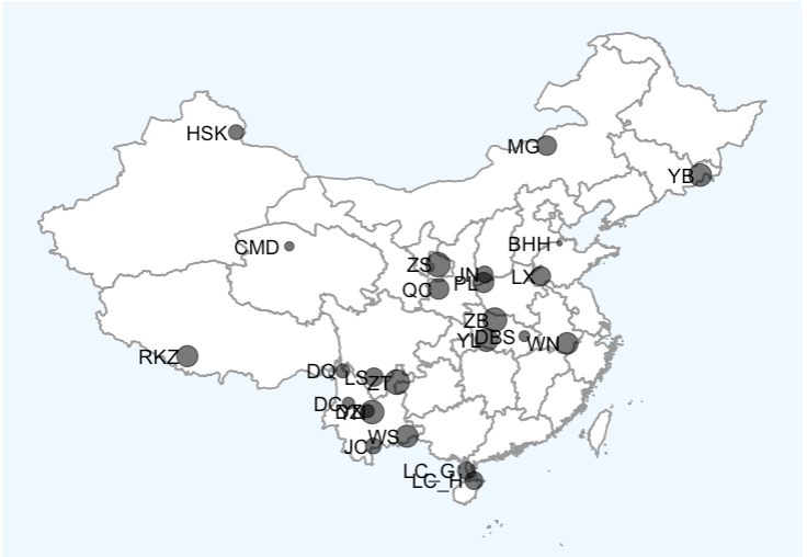
p3 + geom_point(data = data, aes(x = Long, y = Lat, size = Num), alpha = 0.6) + geom_text(data = data, aes(x = Long, y = Lat, label = Bbbr), hjust = 1.2, vjust = 0)
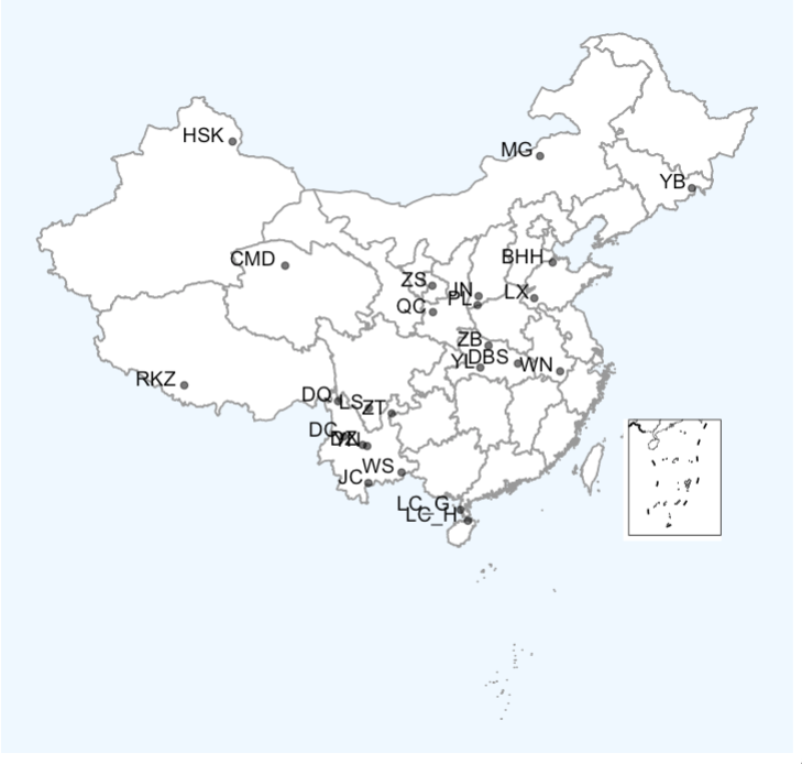
p4 <- p3 + geom_point(data = data, aes(x = Long, y = Lat), alpha = 0.6) + geom_text(data = data, aes(x = Long, y = Lat, label = Bbbr), hjust = 1.2, vjust = 0)
# 画九段线
nine_lines = sf::read_sf('geojson/九段线GS(2019)1719号.geojson')
china = sf::read_sf('geojson/中国省级地图GS(2019)1719号.geojson')
nine_map = ggplot() +
geom_sf(data = china,fill='NA', size=0.5) +
geom_sf(data = nine_lines,color='black',size=0.5)+
coord_sf(ylim = c(-4028017,-1877844),xlim = c(117131.4,2115095),crs="+proj=laea +lat_0=40 +lon_0=104")+ #这是定义九段线的范围,并将投影下的范围改成地理坐标,也可改动里面的范围,选择更合适的九段线范围
theme(
aspect.ratio = 1.25, #调节长宽比
axis.text = element_blank(),
axis.ticks = element_blank(),
axis.title = element_blank(),
panel.grid = element_blank(),
panel.background = element_blank(),
panel.border = element_rect(fill=NA,color="grey10",linetype=1,size=0.5),
plot.margin=unit(c(0,0,0,0),"mm"))
# 合并大小图
ggdraw() + draw_plot(p4) +draw_plot(nine_map, x = 0.78, y = 0.12, width = 0.12, height = 0.5)
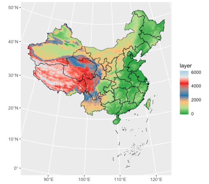
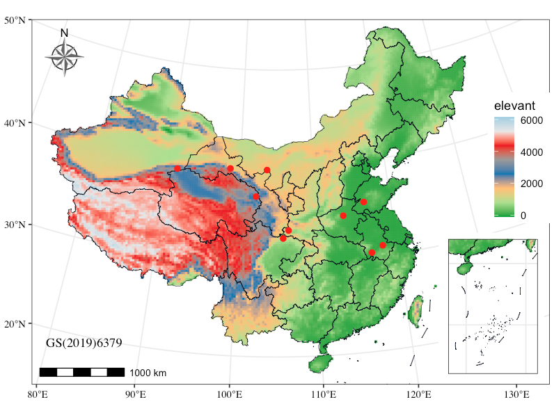
3. 地形图
# 加载R包
pacman::p_load(tidyverse, sf, raster, ggspatial, stars, geoviz, rgeos, sp, rgdal)
# 一定要加载后三个包啊!
# 设置投影
crs_84 <- st_crs("EPSG:4326") ## WGS 84 大地坐标
crs_al <- st_crs("+proj=aea +lat_1=25 +lat_2=47 +lon_0=105") ## Albers Equal Area Conic投影
#地图获取
china_all <- sf::st_read("https://geo.datav.aliyun.com/areas_v3/bound/100000_full.json") %>% st_transform(crs_al)
hainan <-sf::st_read("https://geo.datav.aliyun.com/areas_v3/bound/460000_full.json") %>% st_transform(crs_al)
# 截取地图
tmp_china <- # 去除 海南省,九段线
china_all %>%
filter(!adcode %in% c("460000", "100000_JD")) %>%
st_make_valid() %>%
st_union()
tmp_hainan <- # 海南省去除 三沙市
hainan %>%
filter(!name %in% "三沙市") %>%
st_make_valid() %>%
st_union()
# #### 组合起来中国大陆边框
china_com <- st_union(tmp_china, tmp_hainan)%>% st_as_sf()
#### 海拔获取
dem <- geoviz::mapbox_dem(
lat = 35.8617,
long = 104.1954,
square_km = 2000,
api = "pk.eyJ1IjoiYmVueXNmIiwiYSI6ImNrczBtdWE0ajBwNjcydnBqMjRyZDdsOXkifQ.sUcMdooE7b9uQqzfrnWdSQ"
)
# 备用api: pk.eyJ1IjoibWlzNDE3IiwiYSI6ImNseTlzZDdzNTB2bmMyam9qZnBrNmlma3MifQ.PudTH_3F0M1kDAU-U3twIA
china_dem <- dem %>%
projectRaster(crs = crs_al$wkt) %>% # 修改栅格数据的投影
aggregate(fact = 3) %>% ## 降低分辨率,减少运算量
raster::crop(., raster::extent(china_com)) %>%
raster::mask(china_com) %>%
stars::st_as_stars() %>%
st_as_sf()
# #### 颜色配置
colors <- c(
"#33A02C", "#B2DF8A", "#FDBF6F", "#1F78B4",
"#575c9e", "#837d76", "#7b5c3e", "#E31A1C")
#### 绘制大陆区域
p1 <-
ggplot() +
geom_sf(aes(fill = layer, color = layer), data = china_dem) +
geom_sf(size = .2, fill = "transparent", color = "#060d1b", data = china_all) +
scale_fill_gradientn(colours = colors) +
scale_color_gradientn(colours = colors)
## 截取南海九段线
p2 <-
p1 +
coord_sf(crs = crs_84) + ## 将投影坐标转换为大地坐标
scale_x_continuous(expand = c(0, 0), limits = c(107, 122), breaks = seq(70, 140, 10)) +
scale_y_continuous(expand = c(0, 0), limits = c(2, 24), breaks = seq(10, 60, 10)) +
guides(fill = "none", color = "none") +
theme_bw() +
theme(
axis.text = element_blank(),
axis.ticks = element_blank(),
axis.title = element_blank()
)
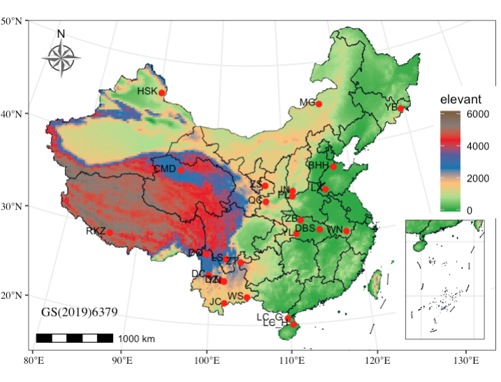
#### 读取采样点数据
# 读入自己的数据
data <- read.csv("sites.csv")
'''
| | | | | |
|---|---|---|---|---|
|Breed|Bbbr|Long|Lat|Num|
|bohaihei|BHH|117.61|37.77|1|
|chaidamu|CMD|94.75|37.55|2|
|dabieshan|DBS|114.64|30.81|3|
|dengchuan|DC|99.76|25.78|4|
|dianzhong|DZ|101.37|25.2|5|
|diqing|DQ|99.27|28.21|6|
'''
#### 图形拼接
p1+coord_sf(crs = crs_al, default_crs = crs_84) + geom_point(data=data,aes(x=Long,y=Lat),color="red",size=2) + geom_text(data = data, aes(x = Long, y = Lat, label = Bbbr), size=3, hjust = 1.2, vjust = 0.2)+
annotate(geom="text",x=80,y=18,
label="GS(2019)6379",family="serif",vjust=0,hjust=0) +
##审图号
scale_x_continuous(expand = c(0, 0),limits=c(72,142),
breaks=seq(70, 140, 10)) +
scale_y_continuous(expand = c(0, 0),limits = c(17,55.5),
breaks = seq(10, 60, 10)) +
labs(fill = "elevant", color = "elevant") +
theme_bw() +
theme(axis.text = element_text(family ="serif",color="black"),
## 字体改为新罗马
axis.title = element_blank(),
legend.position = c(1,0.8),
legend.justification = c(1,1)) +
annotation_scale(location = "bl") +
# 设置距离刻度尺
annotation_north_arrow(
location = "tl",
style = north_arrow_nautical(
fill = c("grey40", "white"),
line_col = "grey20")
) + annotation_custom(ggplotGrob(p2),
xmin= 122,xmax = 138,ymin=15,ymax = 29)
4. 交互式地图
import plotly.express as px
import pandas as pd

df =pd.read_csv("breed_info_map.csv")
df.head()


# 假设你有采样地数据
# columns: latitude, longitude, breed, count

# 使用 scatter_mapbox(交互式地图)
fig = px.scatter_map(
    df,
    lat="Latitude",
    lon="Longitude",
    color="Breed name",                # 按品种区分颜色
    size="Sample size",                 # 数量决定点大小
    hover_name="Breed name",           # 鼠标悬停显示
    hover_data={"Sample size": True, "Latitude": False, "Longitude": False},
    zoom=3,
    height=800,
    size_max=10
)

# 设置地图风格(这里用open-street-map,不需要token)
fig.update_layout(
    mapbox_style="open-street-map",
    title="采样地点分布",
    margin={"r":0,"t":30,"l":0,"b":0}
)

fig.show()


fig.write_html("sampling_map.html", include_plotlyjs="cdn")

