Using PLINK for Genome-Wide Association Study
一、 基本用法
01 assoc
基本的case/control关联,质量性状数量性状均可,不能加协变量
数据过滤
plink --tfile /stor9000/apps/users/NWSUAF/2020060179/Sheep/GWAS/all_sample339.snp.filtered2.final.rename.modified --chr-set 26 --recode transpose --out all_sample339.snp.filtered2.final.rename.modified323.filter --maf 0.05 --geno 0.1 --mind 0.1 --hwe 0.001 --autosome-xy --allow-extra-chr
整理性状
cut -d " " -f 1 all_sample339.snp.filtered2.final.rename.modified323.filter.tfam > samples
for i in `cat samples`; do grep $i /stor9000/apps/users/NWSUAF/2020060179/Sheep/GWAS/trait_tail_type2 >> tail_wool;done
sed -i 's/1$/2/g' tail_wool
sed -i 's/0$/1/g' tail_wool
关联分析
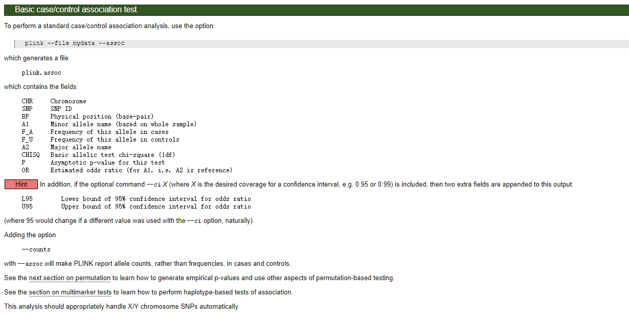
# 质量性状,默认基于卡方检验,
plink --tfile ../all_sample339.snp.filtered2.final.rename.modified323.filter --pheno tail_wool  --assoc --out tail_wool.assoc --chr-set 26 --allow-no-sex
Info
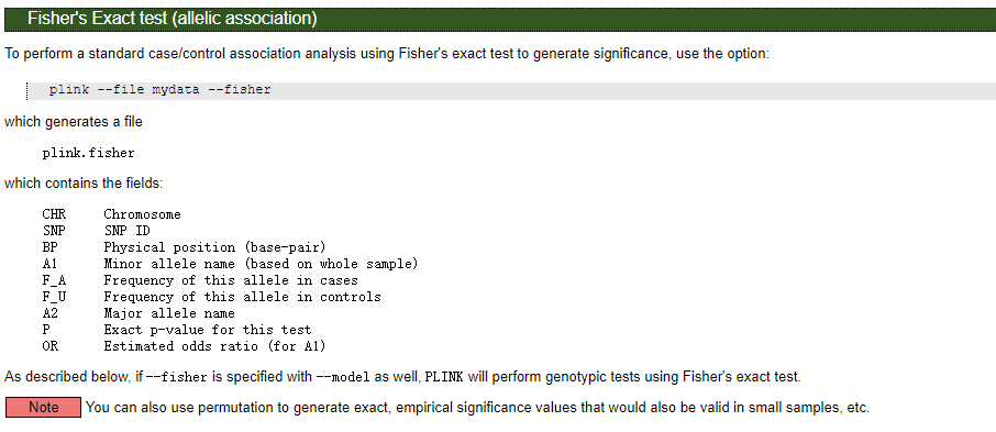
也可以加--fisher进行Fisher精确检验计算精确P值,否则--assoc默认根据chi square分布计算近似P值。
在大样本的情况下(总样本数>40),可以用chi square检验,若总样本数<40,单个最小频数<5,则用fisher检验较为合适。
结果文件格式:
Info
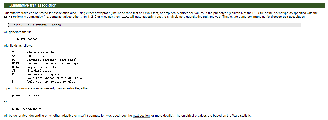
对于数量性状,基于t检验,对于数量性状来说--assoc结果和--linear以及--logistic中的ADD效应的P值一样:
#

plink --tfile ../all_sample339.snp.filtered2.final.rename.modified323.filter --pheno tail_length --assoc --out tail_length.assoc --chr-set 26 --allow-no-sex

# 结果文件格式
Warning
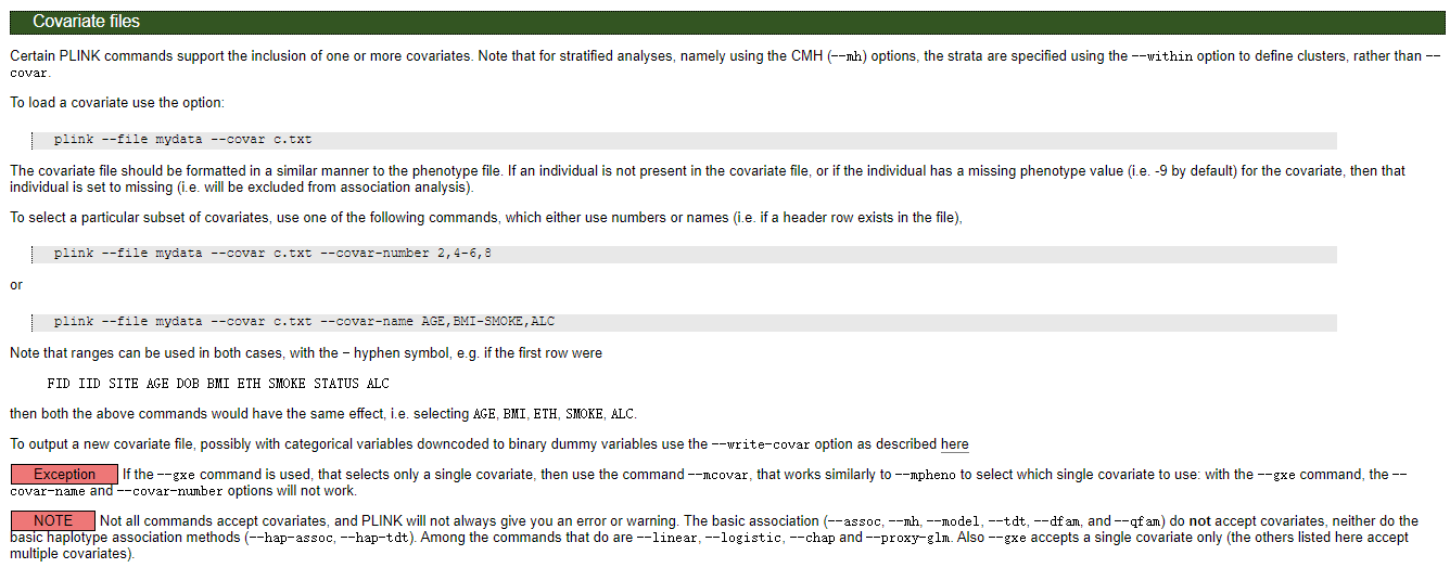
协变量为分类变量时,需要转换为虚拟变量/哑变量
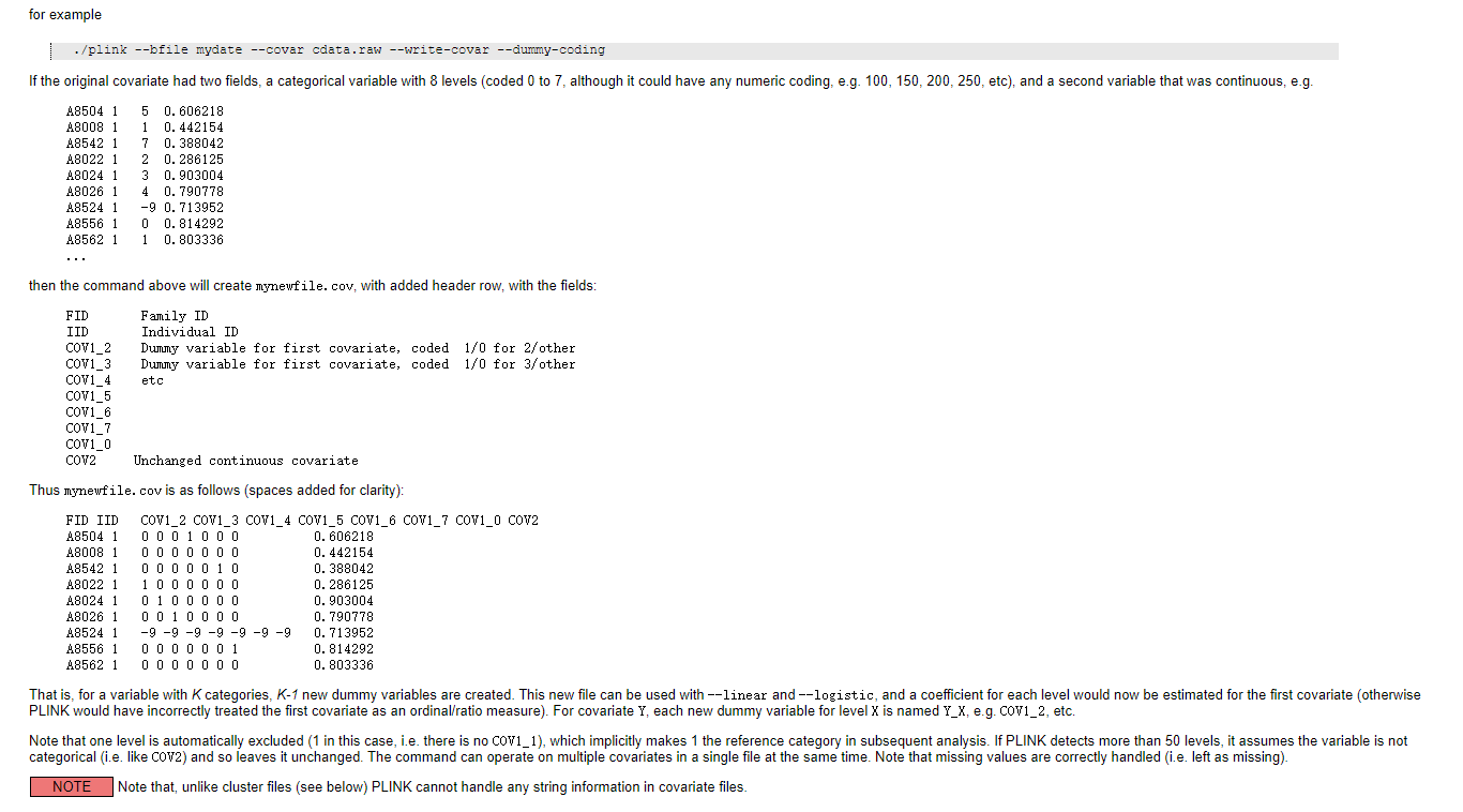
plink --tfile all_sample339.snp.filtered2.final.rename.modified323.filter --covar ../covariate_for_plink --write-covar --dummy-coding --out ../dummy_covariate_for_plink --chr-set 26
02 logistic
**逻辑回归,用于分类变量,可以添加协变量,基于t检验
# PCA结果作为协变量
plink --tfile all_sample339.snp.filtered2.final.rename.modified323.filter  --pca --chr-set 26 --maf 0.05 --out all_sample339.snp.filtered2.final.rename.modified323.filter.pca

# 关联
plink --tfile ../all_sample339.snp.filtered2.final.rename.modified323.filter --pheno tail_wool  --logistic --covar ../covariate_for_plink --out tail_wool.logistic --chr-set 26 --allow-no-sex
03 linear
线性回归,用于连续性变量,可以添加协变量,基于t检验
不加协变量
plink --tfile ../all_sample339.snp.filtered2.final.rename.modified323.filter --pheno tail_length --linear --out tail_length.linear.nocov --chr-set 26 --allow-no-sex
加协变量
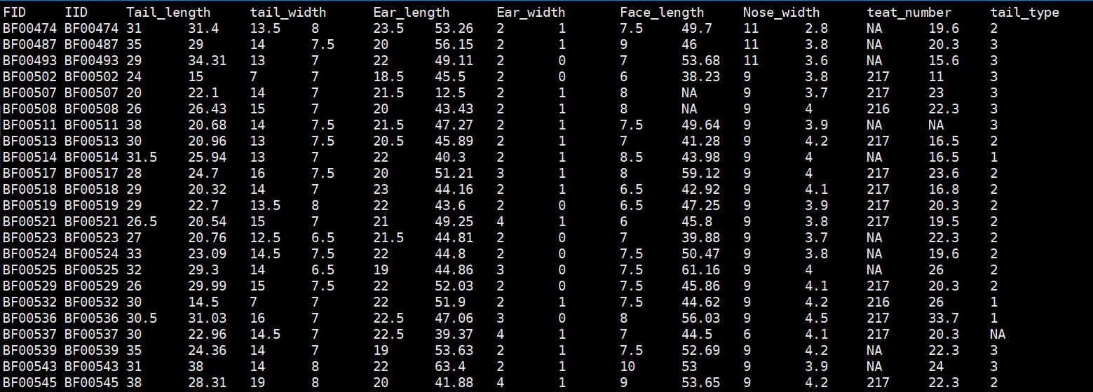
协变量格式:
# 关联

plink --tfile ../all_sample339.snp.filtered2.final.rename.modified323.filter --pheno tail_length  --linear --covar ../covariate_for_plink --out tail_length.linear --chr-set 26 --allow-no-sex

# 可以加上--hide-covar参数,不显示协变量,只显示ADD加性效应。

plink --tfile ../all_sample339.snp.filtered2.final.rename.modified323.filter --chr-set 26 --pheno ../all_phenotypes --pheno-name Birth_weight --linear --allow-no-sex --out birth_weight.linear.cov1 --covar ../covariate_for_plink --hide-covar
二、进阶技巧
01 所有表型一起做
表型文件格式:
Warning
表型中如果用01编码二元分类性状,需要改成其它数字编码
# 关联分析

plink --tfile all_sample339.snp.filtered2.final.rename.modified323.filter --chr-set 26 --assoc --pheno all_phenotypes --all-pheno --allow-no-sex --out allpheno

# 所有表型一起做一般线性模型
plink --bfile /stor9000/apps/users/NWSUAF/2015010726/Sheep/GWAS_for_HuSheep/02.GWAS/by_GEMMA/all_samples317.filter.sort --chr-set 26 --linear hide-covar --pheno /stor9000/apps/users/NWSUAF/2015010726/Sheep/GWAS_for_HuSheep/02.GWAS/all_phenotypes.txt --all-pheno --allow-no-sex --out allpheno --covar covariate_for_plink_pca3_age_sib
02 当有P值为0时,设定最小P值
# --output-min-p 1e-99    # any p-value below 10^{-99} will be reported as 10^{-99}

plink --file /stor9000/apps/users/NWSUAF/2015010726/Sheep/GWAS_for_Black_Suffolk/01.data/plink/Black_Suffolk.snp.filtered --pheno /stor9000/apps/users/NWSUAF/2015010726/Sheep/GWAS_for_Black_Suffolk/02.GWAS/all_pheno_mod.grep --pheno-name Chest_width --linear hide-covar --covar ../../covariates_pca3 --chr-set 26 --allow-no-sex --out Chest_width --output-min-p 1e-99
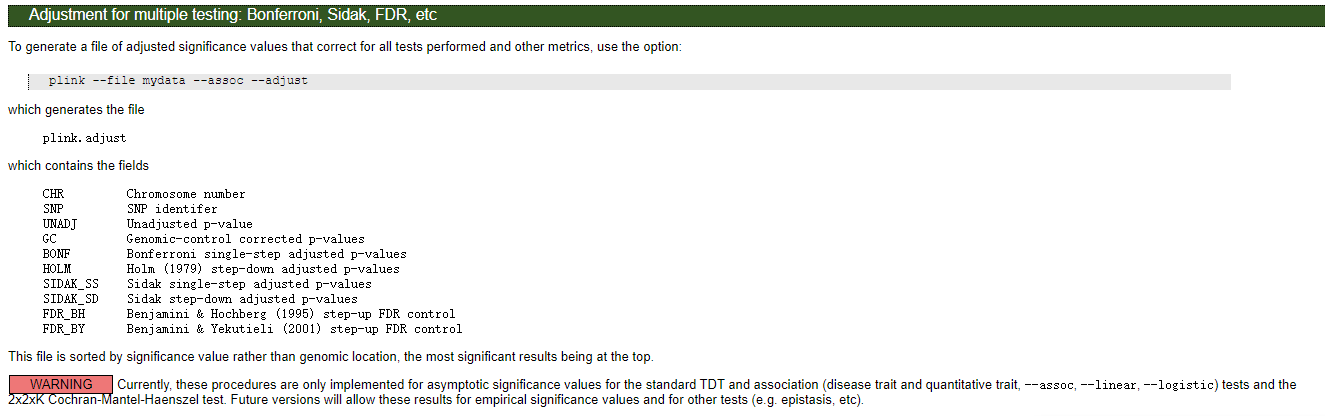
03 加上多重检验的关联分析
Bonferroni校正
plink --tfile all_sample339.snp.filtered2.final.rename.modified323.filter --chr-set 26 --assoc --pheno all_phenotypes --pheno-name tail_type --allow-no-sex --out type --adjust
结果文件格式:
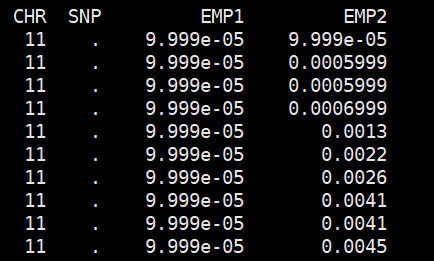
permutation校正
plink --tfile all_sample339.snp.filtered2.final.rename.modified323.filter --chr-set 26 --assoc --pheno all_phenotypes --pheno-name tail_type --allow-no-sex --out type --mperm 10000

# or

plink --tfile all_sample339.snp.filtered2.final.rename.modified323.filter --chr-set 26 --assoc --pheno all_phenotypes --pheno-name Tail_length --allow-no-sex --out Tail_length_msperm --mperm 10000
结果文件
sort -k4,4 -g Tail_length_msperm.qassoc.mperm | head
三、可视化与注释
01 可视化曼哈顿图
提取P值
awk '{OFS="\t"}{print $1,$3,$9}' tail_length.linear.nocov.assoc.linear | grep -v 'NA' > tail_length.linear.nocov.assoc.linear.pvalue.txt
可视化
##可视化
library(qqman)
data <- read.table("C:/Users/Administrator/Desktop/gwas.assoc.txt",header = T) # 读取数去存到data变量里面
colorset<-c("blue4", "orange3") # 创建一个颜色集合
manhattan(data, CHR = "CHR", BP = "bp", SNP = "SNP", p = "P-VALUE", col = colorset)  # 画曼哈顿图

# 或者服务器上一键式
source /stor9000/apps/users/NWSUAF/2015010726/.bashrc
export R_LIBS_USER="/stor9000/apps/users/NWSUAF/2015010726/R/x86_64-conda_cos6-linux-gnu-library/3.5/"
R脚本内容
############################ /stor9000/apps/users/NWSUAF/2015010726/scripts/Manhattan_QQ_plot.R脚本内容#################################
# Object: Manhattan & QQ Plot for genome-wide association study
# Output: Single figure with PDF format
# Authors: Yingwei Guo
# Date: 8th, Jan, 2021
# Usage: Rscript commandArgs()[4] pvalue.txt sites_number traits_name
# 如果报没有qqman这个包的错误,在shell环境运行下面一行命令:
# export R_LIBS_USER="/stor9000/apps/users/NWSUAF/2015010726/R/x86_64-conda_cos6-linux-gnu-library/3.5/"

library(qqman)
args <- commandArgs(trailingOnly = TRUE)
data <- read.table(args[1],header = T) # 读取数去存到data变量里面
colorset <- c("#4C72B0", "#DD8452") # 创建一个颜色集合
pdf(paste0(args[3], ".pdf"), width = 18,height=4.5)
layout(matrix(c(1,2), 1, 2, byrow = TRUE),widths=c(3,1), heights=c(1,1))
par(mar = (c(3,4,2,2)+ 0.5), mgp=c(1.6,1,0))
par(bty="l", lwd=1.5)  ## bty=l  the plot is coordinate instead of box
manhattan(data, CHR = "CHR", BP = "BP", SNP="SNP", p = "P", suggestiveline = F, genomewideline = F, cex = 0.8)  # 画曼哈顿图,默认是黑色和灰色,加color=colorset可自定义
sites_number <- as.numeric(args[2])
abline(h=-log10(0.05/sites_number), lty=5, col="grey40") # 自定义阈值线,h=-log10(0.05/sites_number)
qq(data$P, cex = 0.8)
dev.off()
#############################################################################################################################
用法
Rscript /stor9000/apps/users/NWSUAF/2015010726/scripts/Manhattan_QQ_plot.R P值列不包含NA的GWAS结果文件 位点数 性状名字

例如:

Rscript /stor9000/apps/users/NWSUAF/2015010726/scripts/Manhattan_QQ_plot.R Birth_weight.pvalue.txt 281613 Birth_weight.mht
02 位点过多时的可视化方式(感谢好朋友提醒)
可视化的本质是把每个点以pos为横坐标,以P值为纵坐标标注在坐标轴上。因此,当位点数目超过百万级别时,生成速度很慢,可以用下面的脚本进行可视化。原理大概是,把那些P值不显著有距离相近的位点去除一些,这样在图上显示看起来是一样的。
脚本中定义了一个名为 GAPIT.Pruning 的函数,该函数的主要目的是从大量数据点中筛选出一个子集,以便在绘图时只展示这些代表性点,从而减少绘图的复杂度和时间。
优化后的脚本
##########################################MANHATTAN_QQ.r#######################################
# Object: Manhattan & QQ Plot for genome-wide association study
# Output: Single figure with PDF format
# Authors: Zhiwu Zhang
# Modified by Zhengkui Zhou (zkzhou@126.com)
# Last update: Feb 8, 2014


`GAPIT.Pruning` <-
function(values,DPP=5000){

if(length(values)<=DPP)return(c(1:length(values)))

#values= log.P.values
values=sqrt(values)  #This shift the weight a little bit to the low building.

#Handler of bias plot
rv=runif(length(values))
values=values+rv
values=values[order(values,decreasing = T)]

theMin=min(values)
theMax=max(values)
range=theMax-theMin
interval=range/DPP

ladder=round(values/interval)
ladder2=c(ladder[-1],0)
keep=ladder-ladder2
index=which(keep>0)


return(index)
}#end of GAPIT.Pruning
#=============================================================================================


#Prune most non important SNPs off the plots,
#Object: To get index of subset that evenly distribute
#`GAPIT.Pruning` <-
#function(values,DPP){
#if(length(values)<=DPP)return(c(1:length(values)))
#values=sqrt(values)
#theMin=min(values)
#theMax=max(values)
#range=theMax-theMin
#interval=range/DPP
#ladder=round(values/interval)
#ladder2=c(ladder[-1],0)
#keep=ladder-ladder2
#index=which(keep>0)
#return(index)
#}

`GAPIT.Manhattan` <-
function(GI.MP = NULL, name.of.trait = "Trait",plot.type = "Genomewise", plot.type2 = "Chromosomewise", DPP=50000, cutOff=0.01, band=5, seqQTN=NULL){
print(paste("Start to plot figure for trait: ", name.of.trait ,sep = ""))
if(is.null(GI.MP)) return
P.values <- as.numeric(GI.MP[,3])
borrowSlot=4
GI.MP[,borrowSlot]=0 #Inicial as 0
if(!is.null(seqQTN))GI.MP[seqQTN,borrowSlot]=1

index=which(GI.MP[,borrowSlot]==1  & is.na(GI.MP[,3]))
GI.MP[index,3]=1
GI.MP=matrix(as.numeric(as.matrix(GI.MP) ) ,nrow(GI.MP),ncol(GI.MP))

#Remove all SNPs that do not have a choromosome, bp position and p value(NA)
GI.MP <- GI.MP[!is.na(GI.MP[,1]),]
GI.MP <- GI.MP[!is.na(GI.MP[,2]),]
GI.MP <- GI.MP[!is.na(GI.MP[,3]),]

#Remove all SNPs that have P values between 0 and 1 (not na etc)
GI.MP <- GI.MP[GI.MP[,3]>0,]
GI.MP <- GI.MP[GI.MP[,3]<=1,]

GI.MP <- GI.MP[GI.MP[,1]!=0,]

numMarker=nrow(GI.MP)
bonferroniCutOff=-log10(cutOff/numMarker)

#Replace P the -log10 of the P-values
GI.MP[,3] <-  -log10(GI.MP[,3])

y.lim <- as.integer(ceiling(max(GI.MP[,3])))
#y.lim = y.lim+1
print("The max -logP vlaue is")
print(y.lim)

chm.to.analyze <- unique(GI.MP[,1])
chm.to.analyze=chm.to.analyze[order(chm.to.analyze)]
numCHR= length(chm.to.analyze)

if(plot.type == "Genomewise")
{
nchr=max(chm.to.analyze)
ncycle=ceiling(nchr/band)
ncolor=band*ncycle
palette(rainbow(ncolor+1))
cycle1=seq(1,nchr,by= ncycle)
thecolor=cycle1

for(i in 2:ncycle){thecolor=c(thecolor,cycle1+(i-1))}
GI.MP <- GI.MP[order(GI.MP[,2]),]
GI.MP <- GI.MP[order(GI.MP[,1]),]
color.vector <- rep(c("orangered","navyblue"),numCHR)
ticks=NULL
lastbase=0

#change base position to accumulatives (ticks)
for (i in chm.to.analyze)
{
  index=(GI.MP[,1]==i)
  ticks <- c(ticks, lastbase+mean(GI.MP[index,2]))
  GI.MP[index,2]=GI.MP[index,2]+lastbase
  lastbase=max(GI.MP[index,2])
}
x0 <- as.numeric(GI.MP[,2]) ## BP
y0 <- as.numeric(GI.MP[,3]) ## P
z0 <- as.numeric(GI.MP[,1]) ## CHR
position=order(y0,decreasing = TRUE)
#print(length(position))
index0=GAPIT.Pruning(y0[position],DPP=DPP)
index=position[index0]
x=x0[index]
y=y0[index]
z=z0[index]
output=cbind(z,x,y)
#print(output)
#write.table(output, paste("gwasplot.","printy",".txt",sep=""), sep = '\t', row.names = F, col.names = T, quote = F)
#Extract QTN
QTN=GI.MP[which(GI.MP[,borrowSlot]==1),]

#Draw circles with same size and different thikness
size=1
ratio=5
base=1
themax=max(y)
themin=min(y)
wd=((y-themin+base)/(themax-themin+base))*size*ratio
s=size-wd/ratio/2
y.lim <- as.integer(ceiling(max(GI.MP[,3])))
#y.lim = 10
  pdf(paste("GWAS.", name.of.trait,".Manhattan-QQ Plot.pdf" ,sep = ""), width = 18,height=4.5)
  layout(matrix(c(1,2), 1, 2, byrow = TRUE),widths=c(3,1), heights=c(1,1))  ##
  par(mar = (c(3,4,2,2)+ 0.5), mgp=c(1.6,1,0))   ##
  par(bty="l", lwd=1.5)  ## bty=l  the plot is coordinate instead of box
  mycols=rep(c("orangered","navyblue"),max(z))  ## doulb dolor loop by chromosome
plot(y~x,ylab=expression(-log[10](italic(p))) , ylim=c(0,y.lim), xaxs="i", yaxs="i" ,
     cex.axis=0.5, cex.lab=1.0 ,col=mycols[z], axes=FALSE, type = "p",
     pch=20,lwd=wd,cex=0.5, xlab="Chromosome")
if(!is.null(dim(QTN)))abline(v=QTN[,2], lty = 2, lwd=1.5, col = "grey")
abline(h=bonferroniCutOff,col="dimgray",lty=2, lwd=1)
title(xlab="Chromosome")
 axis(1, at=ticks,tck=-0.01, cex.axis=1,labels=chm.to.analyze,tick=T, lwd=1.5, padj=-1)    ## lwd: line width tick=T,
 axis(2, tck=-0.01, cex.axis=1,lwd=1.5, padj=1)     ## tck=-0.01 let the tck shor
 box()
 mtext(paste("GWAS on ",name.of.trait, sep=""), cex=1.5, font.main =1,  side=3, outer=TRUE,line=-1.5)
print("Manhattan-Plot.Genomewise finished!")

############# QQ-plot#################
DPP=50000
if(length(P.values[P.values>0])<1) return(NULL)
DPP=round(DPP/4) #Reduce to 1/4 for QQ plot
P.values <- P.values[order(P.values)]
p_value_quantiles <- (1:length(P.values))/(length(P.values)+1)
    log.P.values <- -log10(P.values)
    log.Quantiles <- -log10(p_value_quantiles)
    index=GAPIT.Pruning(log.P.values,DPP=DPP)
    log.P.values=log.P.values[index ]
    log.Quantiles=log.Quantiles[index]
    qqplot(log.Quantiles, log.P.values, xlim = c(0,max(log.Quantiles)), ylim = c(0,max(log.P.values)),pch=20, mgp=c(1.6,0.5,0),
           cex.axis=1, cex.lab=1, lty = 1, lwd = 1.2, col = "Blue" ,xlab =expression(Expected~~-log[10](italic(p))), tck=-0.015,
           ylab = expression(Observed~~-log[10](italic(p))))
    abline(a = 0, b = 1, col = "red")
dev.off()
print("QQ-Plot finished!")
print(paste("Manhattan & QQ Plot for trait: ", name.of.trait," accomplished successfully!" ,sep = ""))
}
}
用法
Rscript MANHATTAN_QQ.r gwas_results.txt "TraitName"
03 位点注释
for i in Birth_weight Ear_length Ear_width Nose_width tail_circumference Tail_length teat_number ; do sed -i 's/^27/X/' $i.top;done

for i in Birth_weight Ear_length Ear_width Nose_width tail_circumference Tail_length teat_number ; do cut -f 1-2 $i.top |bcftools view -R - /stor9000/apps/users/NWSUAF/2020055372/sheep_data/call_VCF/all_sample339.snp.filtered2.final.rename.vcf.gz -Oz -o $i.top.vcf.gz ;done

for i in Birth_weight Ear_length Ear_width Nose_width tail_circumference Tail_length teat_number ; do perl /stor9000/apps/users/NWSUAF/2015010726/software/annovar/table_annovar.pl -buildver OAR4.0 -protocol refGene -operation g -vcfinput $i.top.vcf.gz  /stor9000/apps/users/NWSUAF/2015010726/Sheep/reference/Oar4.0/annovar_db/ -outfile $i.top; done

for i in Birth_weight Ear_length Ear_width Nose_width tail_circumference Tail_length teat_number ; do sed '1d' $i.top.OAR4.0_multianno.txt | cut -f 1-2,4-10 |csvtk join -t -f "1,2;1,2" -k $i.top - -T > $i.p_anno.txt;done